


This Little LSE Went to Market...
The structure of US organized real time wholesale electricity markets and their relationship to grid operation

US electricity markets are complex. Some time ago I constructed some diagrams to show electricity market structure and components and there was so much to depict that it took two diagrams to show just the essentials. These diagrams are Entity-Relationship (E-R) diagrams, a documentation form that has been used in computer science as a precursor to database design. In 2008, I adapted this form to illustrate structure in electric power systems, starting with industry structure, but expanding to all grid structure types from there. In E-R diagrams, a box represents a class or type of entity, not a specific organization or system (unless the class has only one member). This means that any particular box may represent many instances of that type. So for example, a box labeled “home” can represent a large set of homes. Lines represent relationships between entities. In my diagrams I label the lines with a word or phrase plus an arrow. This makes it possible to read the diagram as a group of sentences by following the direction of the arrow. For example (see below), ICE operates an exchange. In the case of a bilateral relationship, two arrows are present so the sentence can be read in either direction. Cardinality symbols (“crow’s feet”) at the ends of the lines indicate entity multiplicity (one and only one, one or more, many, etc.)
Figure 1 is the E-R diagram for US electricity market structure. It shows market participant entity classes in relation to the major market classes.
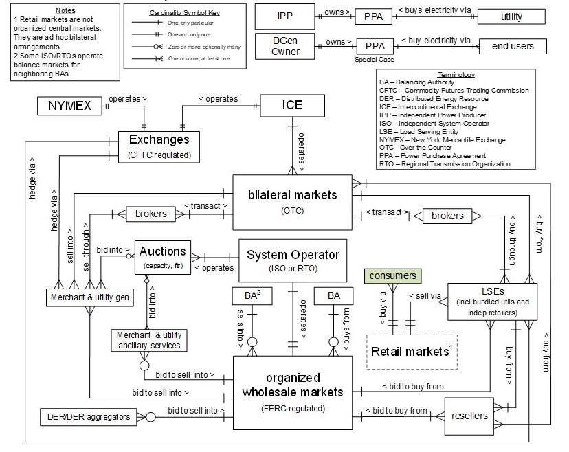
Figure 2 is the E-R diagram for electricity market components (markets, market products, and other outputs) in relation to market participants.
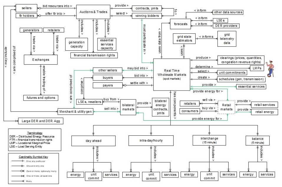
Note in particular the real time wholesale markets, the set of market product components in the lower middle and right of the diagram, and the Locational Marginal Prices (LMPs), if you can spot them (they are right next to Waldo).
Relationship to Grid Operations
Organized real time wholesale electricity markets do not exist everywhere in the US, but where they do, they are integrated with grid operations in several ways.
In tertiary generator control, real time markets are used as the optimization elements of model predictive/receding horizon controls for both balance and interchange. A similar method is used for the day-ahead and intra-day hourly dispatch schedules that are sent to bulk power system generators. Thus, the real time markets are essential elements of bulk power system operations and are integrated with generator control.
A second way that organized real time wholesale markets are connected to grid operations is that they generate Locational Marginal Prices (LMPs). LMPs are the mechanism that connects grid physics to market operations. Without LMPs, early electricity markets caused massive congestion on transmission lines. LMPs serve to create adjustments in power generator bids into the markets and dispatches in a way that avoids the congestion issues.
Figure 3 is a slightly more detailed version of the load-following grid control schema I outlined in my previous post Better Balance Than Simone Biles: Bulk Power System Control Then and Now. In this figure, the primary, secondary, and tertiary generator controls are indicated. Note that in the tertiary control, there are two market-based processes, one for balance inside the Balancing Area (BA), and one for interchange with neighboring BAs. Balance is implemented as a real time market/model predictive control (that is, receding horizon control) operating on a five minute cycle and interchange is done the same way on a 15 minute cycle.
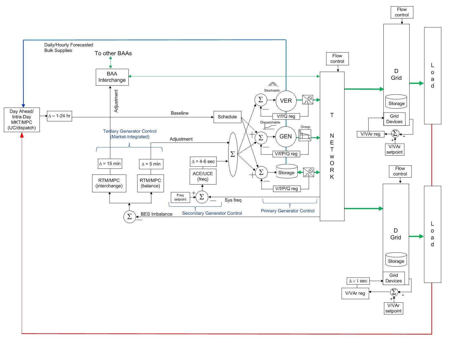
Load and generation data are input to a market process that sets the day-ahead and intra-day hourly generator forward schedules, completing the load-following control. Those market processes are also model predictive/receding horizon processes.
Some Examples of Integrated Electricity Market/Grid Controls
Let’s look at three examples of how this is actually done. Below I have provided process flow models I created for three different US system operator bulk power system generator market-control systems. Terminology varies somewhat by jurisdiction. Note that in these three diagrams, flow is from right to left. This is because they were extracted from larger diagrams in which the market-control system was shown as a feedback mechanism around the whole regional grid system dynamic model. In each case, the System Operator is also a Balancing Authority and so performs the secondary generator control (ACE).
Figure 4 shows a day-ahead process, an interchange process, a balance process, and the ACE process (the intra-day process is not shown for this diagram). Note the N-step ahead calculation, followed by a single time step execution, before the process repeats in a continuous loop. The Secondary Generator Control (ACE) loop runs separately on a four second cycle. Real time LMPs are updated on the 5 minute Balance cycle.
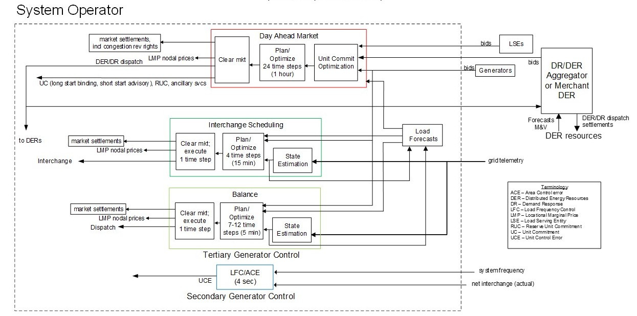
Figure 5 shows a slightly different arrangement for essentially the same processes. In this case, the tertiary control is integrated with the ACE process that runs on a six second cycle.
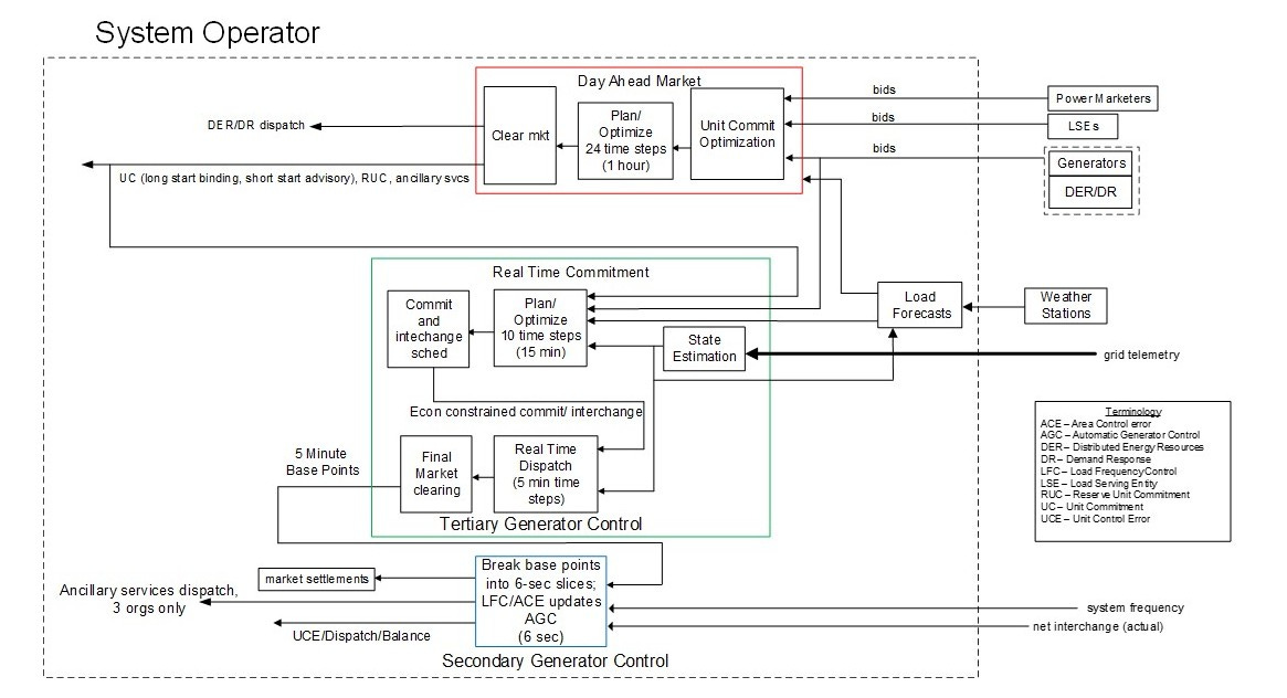
Figure 6 shows an arrangement where energy is handled via a market but power (balance and interchange) are not. Balance and interchange are handled via a non-market process called Security Constrained Economic Dispatch (SCED). Secondary generator control (ACE) is a separate process operating on a four second cycle.
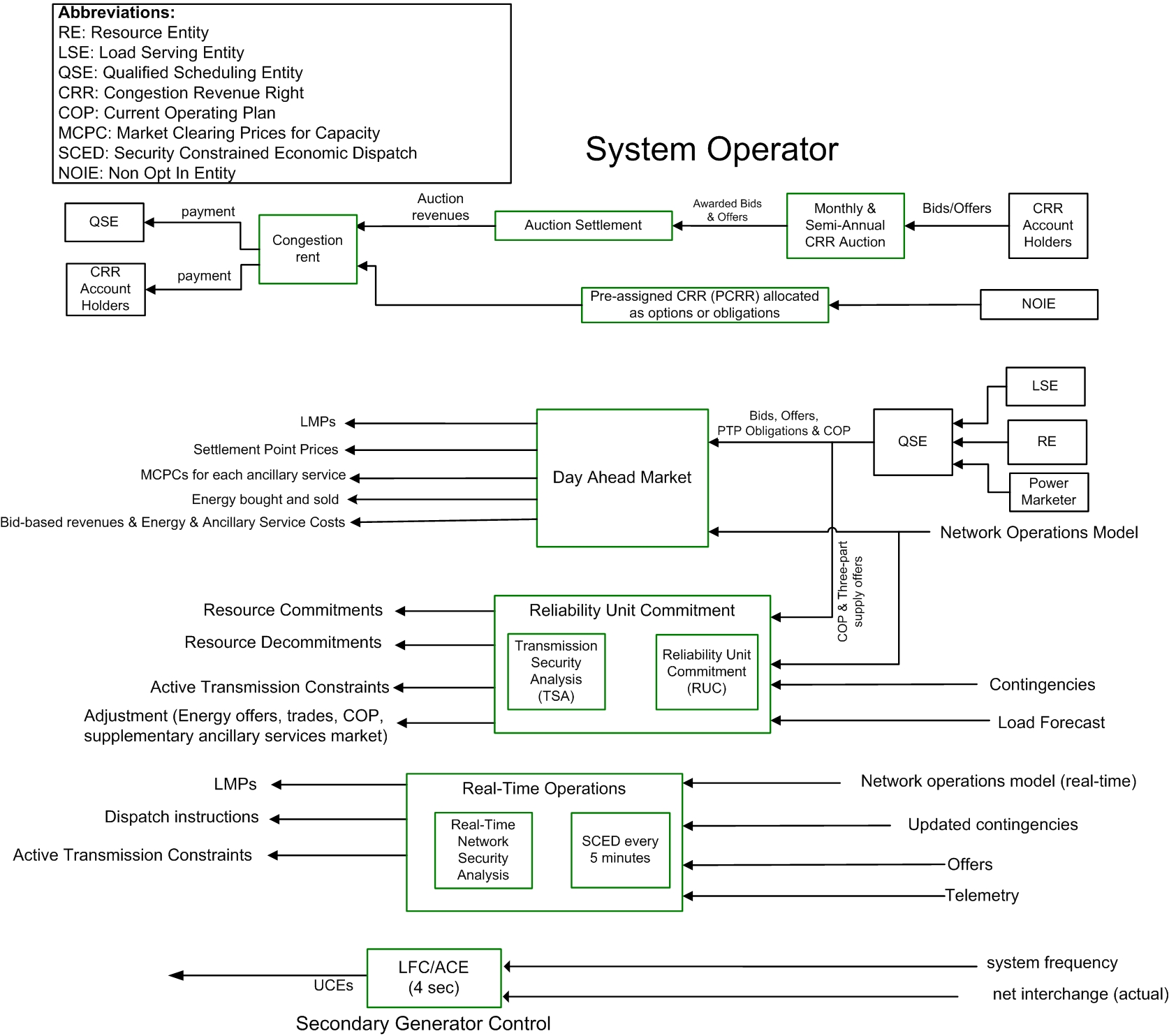
As mentioned, not all parts of the US have independent system operators or regional transmission operators and organized wholesale real time electricity markets. The Security Constrained Economic Dispatch method mentioned in Figure 6 has been used in non-market regions to perform essentially the same functions of committing and scheduling generators as the markets accomplish. SCED is an optimization process that takes into account the costs of operating the generators along with various operating constraints.
This brings us to an interesting point: there is a debate about the two approaches - markets vs. controls. In Electric Grid Market-Control Structure I said the two arguments go like this:
The market view: markets can manage all grid functions. Just get the right market rules and right price signals and everything will work efficiently and reliably.
The control view: controls can manage all grid functions. Just set up and solve the right optimization equations and everything will work efficiently and reliably.
The mathematical methods and solution tools used by electric grid market operators are essentially the same as those used in optimal control methods. This is not really surprising; both have roots in optimization theory and represent formulations of similar or even the same problem from slightly different points of view. Dispatch problems can be and are solved today using either market methods or optimal control methods. At a mathematical level, the formulations are essentially equivalent.
As an example, consider the unit commitment problem. A few decades ago operators used fixed priority orders for unit start-up and shutdown. This evolved into dynamic priority order and, in 1996 the standard became dynamic priority order sequential bidding. Enhanced Lagrangian relaxation was introduced in 2001 to support this optimization, and mixed-integer programming came into use in 2003. In 2013, market optimization benefited from AIMMS 3.13 (Advanced Interactive Multidimensional Modeling System, a software package designed to model and solve large-scale optimization and scheduling problems) and CPLEX 12.5 (an optimization software package accessible through AIMMS). These approaches and tools will be very familiar to control engineers who use optimal control methods.
Markets are presumed to operate voluntarily and do not take into account physical system behavior; no methods exist to derive market rules from a physical system model or to ensure the “right” set of prices will be determined by a market. Controls are presumed operate imperatively and do not take into account human behavior; no methods exist to derive controls from a human system model or to ensure that the “right” set of behavioral incentives will be determined by a control system. A deep examination of markets and controls as applied to power grids at the bulk system shows more similarities than differences and also shows that they are essentially complementary in nature, suggesting that they can and should compensate for each other’s limitations.
That being said, it is clear that markets and controls do not apply equally to all grid management problems. I created a diagram (see Figure 7) to help illustrate where each applies well as a function two variables: latency bound and number of elements involved.
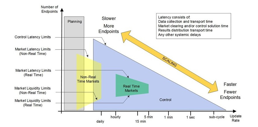
With the increasing penetration of variable energy resources at the distribution level, dynamics are shifting to faster time scales, such that at the distribution edge we must employ controls rather than markets. As update rates increase, each control must be closer to the edge, and control fewer devices until we reach a limit where each control handles only one device (in other words, they operate autonomously). This is an example of a situation where the system triangle comes into play (Centralized and Distributed are Not Polar Opposites).
Many schemes are being proposed and trialed for how to marketize distributed energy resources at regional scale, from wholesale market participation, to per-to-peer energy transactions, to distribution level markets. Significant architectural issues arise from such schemes, but that is a topic for another day.