


Better Balance Than Simone Biles: Bulk Power System Control Then and Now
And what to do about the disruptive effects of wind and solar

Your Father’s Power Grid
Our electrical grids were developed in the 19th and 20th Centuries to be powered by a set of rotating machine electrical generators connected to transmission systems and thence to distribution systems to deliver electricity to the users. The collection of generators and transmission lines plus associated equipment are what we call the Bulk Power System (BPS) or sometimes the Bulk Energy System (BES) and the control systems that evolved to deliver electricity reliably and smoothly are amazingly clever. Here we take a look at how this works, keeping in mind that our grids still mostly work this way even thought some changes are developing due to introduction of Variable Energy Resources (VER) - meaning mainly wind and solar. More about that later. For now, let’s see how “traditional” BPS electrical generation is controlled. There are many more control functions in the grid that what we will examine here (see later) but let’s look at generator control for now.
First, it is important to understand that traditional generator control is a feedback control. Figure 1 shows a vastly simplified control system block diagram for how this works.
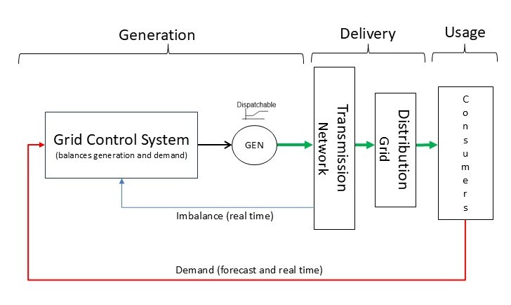
The entire system has (in this diagram) three main parts: the grid control system and generators, the electricity delivery system (transmission and distribution - basically the wires), and most importantly, the consumers (our homes, businesses, factories, street lights, … everything). The control system tells the generators what to do, but how does it know what that is?
We need to do a little sidebar here about feedback control systems. Such controls come in three basic forms:
state regulator - a control that brings the system state to zero and keeps it there or returns it there in spite of perturbations (like balancing a broom upside down on your hand to keep the angle between the broom handle and vertical at zero)
servomechanism - a combination of state regulator plus a reference (setpoint) input to make a system move to and stay at a particular state (think automobile cruise control that keeps the car moving at a fixed speed set by the driver)
tracking control - a control that causes a system to follow something external (think a tracking antenna, which automatically points at all times at a moving object, such as an aircraft)
Looking back at Figure 1, we can see that traditional grid generator control in the large is in fact a tracking control, where the generators are controlled to produce power that tracks electric demand from the consumers. In the power industry, this is called load following, for the reason that customer demand is treated as external to the grid and generation is controlled to follow load closely (yeah, utility folks refer to the customers as “load”). This means that the primary signal that drives the grid is the demand that we the users call for by turning things on (the red arrow) and as a practical matter, the control system uses measures of imbalance between generation and load to ensure tight balance. It is the consumers that tell the grid what to do. This is an important point to remember for later.
So how is this continual balance accomplished when we consumers are always turning things on an off?
First, let’s see how a traditional rotating machine synchronous generator operates. Figure 2 shows the internal controls of such a generator.
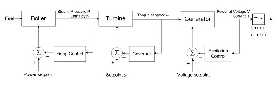
This local (right at the power station) control has four stages. For a thermal generator, the first stage is a servo control loop that controls the rate at which fuel (coal, oil, natural gas) is burned to generate steam to turn the turbine. In a hydro-generator this stage controls the flow gate that determines much water flows through the turbine; in a nuclear reactor this stage controls the control rod positions to set the amount of nuclear flux, which then determines the heat output of the reactor to make steam to turn the turbine.
The second stage servo control regulates the speed at which the turbine turns, which has the effect of setting the frequency of the voltage to be generated (60 Hz in the US).
The third stage controls the field excitation of the generator, which sets the generator output voltage (the frequency having been determined by the second stage and the power level having been set by the first stage).
The fourth stage (droop control) senses power line frequency (also called system frequency) and adjusts the generator frequency and power output. We shall see why this is important shortly.
Thus far, our power grid, with multiple distribution systems attached to a transmission system, looks like Figure 4.
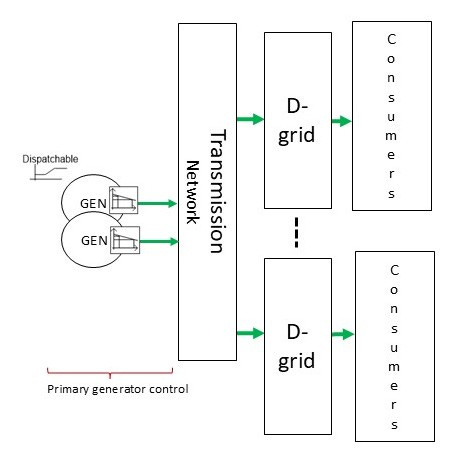
Control at the generator plant is called primary generator control. Note that in the diagram, the generators are denoted as “Dispatchable.” This is because we can set the power output (as well as frequency and voltage) - an important point because dispatchability is crucial to the entire grid control scheme. Remember that we are assembling a tracking control, so we must be able to adjust generator output to follow (track) demand.
But where do the commands to the generators come from? To answer that, we need three more levels of control. We will build them up one at a time, but before we do that, let’s look at why we need the droop controls at the generators.
When multiple rotating machine generators are all connected to a transmission system, they interact with each other. The electromechanical physics is complicated and we are not going to do the math here, but one of the issues is that the total load must be allocated to the generators in proportion to their individual capacities (which are not equal). If this is not done, one generator can be subject to more load than it can handle and it will trip offline. Then the next generator will then have too much load and it will trip, too. A cascading failure will result and the entire system will collapse, creating the dreaded wide area blackout. So the load allocation must be maintained regardless of changes in demand or supply. This called load sharing.
The way that load sharing is done automatically is extremely clever. When there is an imbalance between generation and load, system frequency will deviate from the nominal value (60 Hz in the US). This imbalance may be due to a sudden decrease in demand caused by a transmission line outage, or sudden loss of a generator, for example. When generation exceeds demand, the system frequency rises and when demand exceeds generation, system frequency drops.
The droop controls at each generator sense line frequency locally and adjust the generator power and frequency. Collectively, the entire set of droop controls for all the generators, interacting through grid physics only, finds a new equilibrium system frequency that all the generators settle to, with a new allocation of loads to generators that aligns with individual generator capacities, so load sharing is re-established quickly. This is done automatically, without any centralized control or communication among the generators. Amazing!
But this raises a new issue: we want to get the system back to its nominal system power balance and system frequency after a shift occurs. This is where the next level of control comes in. Figure 5 adds in this next level to our model.
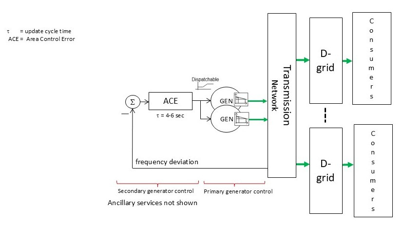
This level of control, called secondary generator control, uses system frequency deviation as the error signal input to a control process called Area Control Error (ACE). ACE controls are closed loop controls that act to adjust generator setpoints to reestablish balance and system frequency. This is often called frequency regulation but it is important to understand the frequency regulation itself, which important, is secondary to the function of “trimming” generator setpoints to address imbalance. ACE controls are implemented by entities known as Balancing Authorities (BAs), each of which performs this function for a specific balancing area. There are many BAs in the US, and each implements the ACE control in a centralized fashion for its respective balancing area, as well as managing power interchanges with neighboring BAs (remember, everybody is connected through the transmission grid). Figure 6 shows the actual ACE control.
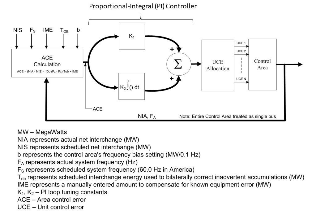
The BA calculates the total Area Control Error, then breaks that down into individual Unit Control Errors that are sent as commands to the generators, causing adjustment in generator setpoints. Communication links are used to do this and the BA updates commands to the generators in its balancing area every 4-6 seconds, depending on the individual BA. Once again, the generators must be dispatchable to do this. Note that while the overall grid control is a tracking control, ACE is essentially a servo control as regards frequency.
But wait, there’s more!
Secondary generator control addresses short term adjustments in the generators in a given balancing area, but longer term balancing must also be addressed and power interchanges occur between BAs and between whole regional grids. So yet another level of control is used to handle this. Figure 7 adds in this level.
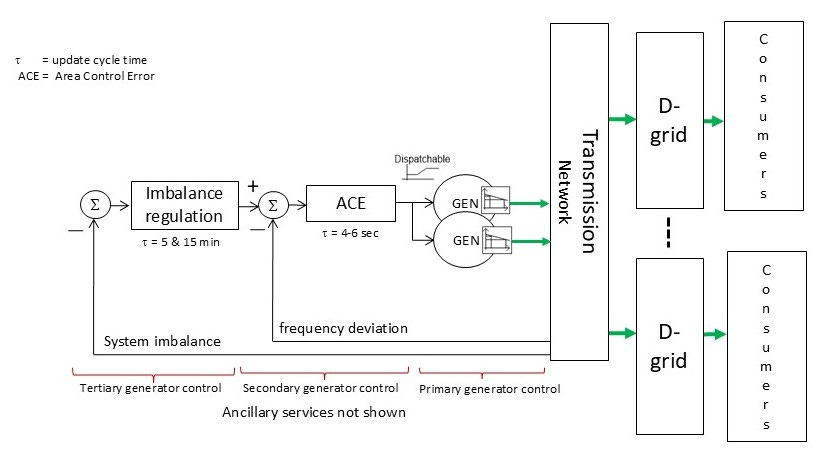
This loop, called tertiary generator control, has two processes. One is for imbalance, and typically runs on a 5 minute cycle of generator adjustments. The other is for interchange adjustments with other BAs, and typically runs on a 15 minute cycle.
We are getting closer, but we are not there yet.
Everything in the primary, secondary, and tertiary generator controls is about making incremental adjustments, but where does total demand come in? Have a look at Figure 8.
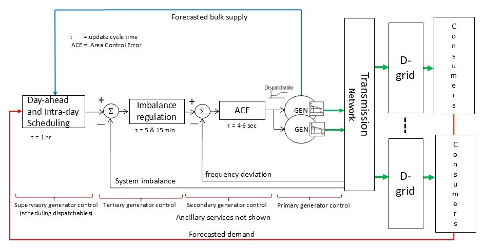
The last and slowest stage of the control is a set of scheduling processes. These processes run from day-ahead hourly schedules to intra-day hourly schedule adjustments. The schedules here are lists of generator power output setpoints over time. These are transmitted to the generators in advance of the actual time periods to which they apply. They constitute the baseline power operating plans for the relevant time periods. Note that these schedules are computed using forecasted and real time (measured) demand, combined with forecasted and real time available bulk generator supply.
The day ahead/intra-day intra-day processes and the balance and interchange processes all use a control method known in other industries (but not in the power industry) as model predictive receding horizon control. This means that the setpoints or adjustments are computed for several future time steps. Then exactly one time step is executed and the entire process is re-computed on a sliding time window basis. In the cases of balance and interchange, the controls seeks to drive incremental imbalance to zero, and so act as state regulators. The scheduling processes act as the overall tracking control.
So, compare Figure 8 to Figure 1 and now you have a decent grasp of how things work in the grid under normal conditions. There is a lot more to all this that I have not covered (see below), but full details would take lots more space than we have here. Once you understand Figure 8, you understand the grid better than almost everybody.
Except…
Except things don’t stay the same forever. We are well into the 21st Century and new kinds of generation are being used at the BPS level (we are not talking about the changes at the distribution system here - that is a big topic for another day).
Side A: Blowin’ in the Wind / Side B: Here Comes the Sun
The introduction of wind and solar power at grid scale (wind and solar farms) is not aligned with this approach to controlling the power grid. Figure 9 below shows an example of wind power hourly variations over a number of days. Nothing smooth about that.
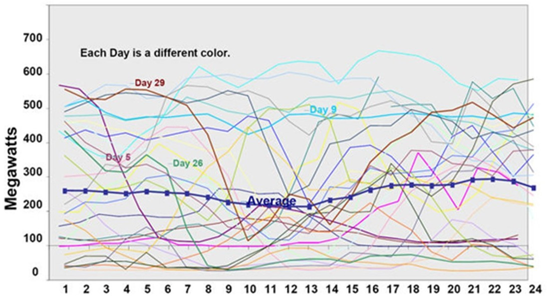
Figure 10 shows solar power volatility over the course of a particular day. Again, not too smooth. Rooftop solar can also make the load apparent to the grid vary randomly as well.
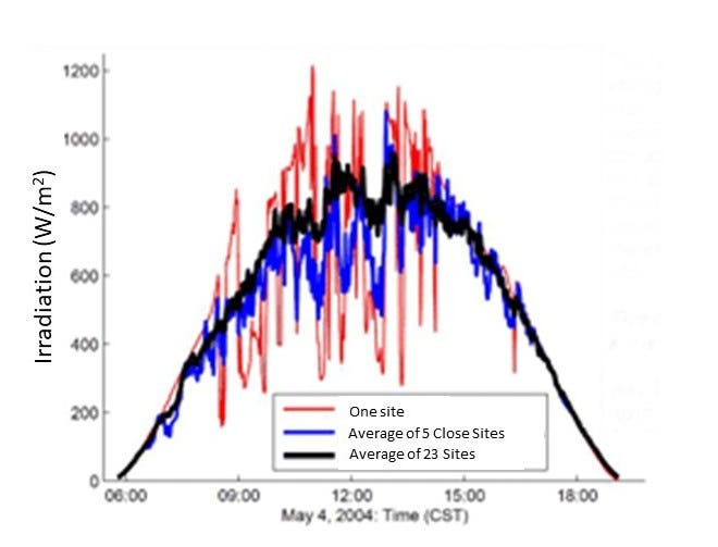
This kind of power injection creates problems: it is not dispatchable as conventional generation is and it can be highly volatile on short time scales. Solar and wind power injection can be curtailed, but the owner/operators of these assets in the US object to curtailment, as it negatively impacts their revenues and production tax credits. So, increasing penetration of solar and wind power increasingly destabilizes the electric power grid. In the Pacific Northwest, it was common to use modulation of hydro-generation (which can be done fairly quickly) to counterbalance fluctuations in wind power. However, the amount of compensation capacity available this way has long since been used up.
To deal with this problem, some utilities are now adding bulk energy storage to the BPS. This is fast, bilateral (two-way) storage, which has been used like generators that can have negative output (meaning it can absorb power from the grid).
With the introduction of grid-scale transmission connected solar and wind farms, and bulk energy storage, the BPS control looks like Figure 11.
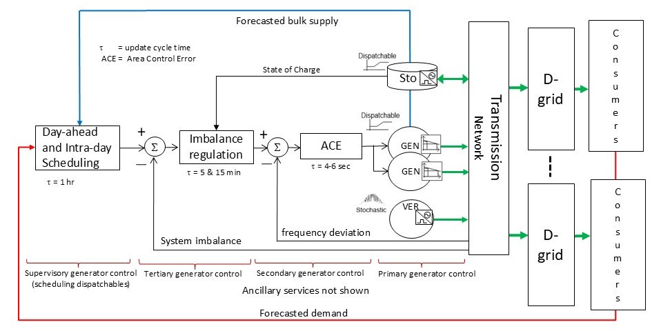
Bulk storage is dispatchable (good) but both storage and VER must interface to the grid via power electronic inverters, unlike conventional generators. Efforts have been made to use storage to counter VER volatility, as well as supply various ancillary grid services.
There is a better way.
I’m Shocked, Shocked! (Yes, I just watched Casablanca the other day)
What we need here is a ♫ smooth operator, smooooth operator♫ . Ahem. Somebody call Sade Adu.
If solar and wind are to be significant components of the power grid, we need to use storage not as a generator or grid services device, but as a shock absorber. Read about this concept in detail in The Grid Needs Shock Absorbers.
Final Comment - Not Your Father’s Power Grid
It has been suggested that we should convert our power systems from load-following to generator-following so as to use just VER (wind and solar). This would mean that VER would free run, and consumer use of electricity would be controlled to fit the available VER outputs. In other words, the grid would tell the consumers what to do instead of the other way around. The consumers would become a system to be servo-controlled by the grid, setting demand to match available (now external to the grid ) supply. Consider how much of the above control structure would have to change to do this. Consider the reactions of consumers as they are told when they may and may not have electricity.
Afternote
The grid control depiction shown above is quite high level and leaves out many elements and details. I would have posted a more detailed diagram but that would have take this post over the email length limit. This post does not show the relationship to multi-time-scale planning processes or organized wholesale electricity markets. It does not address ancillary services or distribution level control. The table below (not guaranteed to be complete) is a more comprehensive list of control functions a power grid needs, including the ones discussed above and others not addressed here.
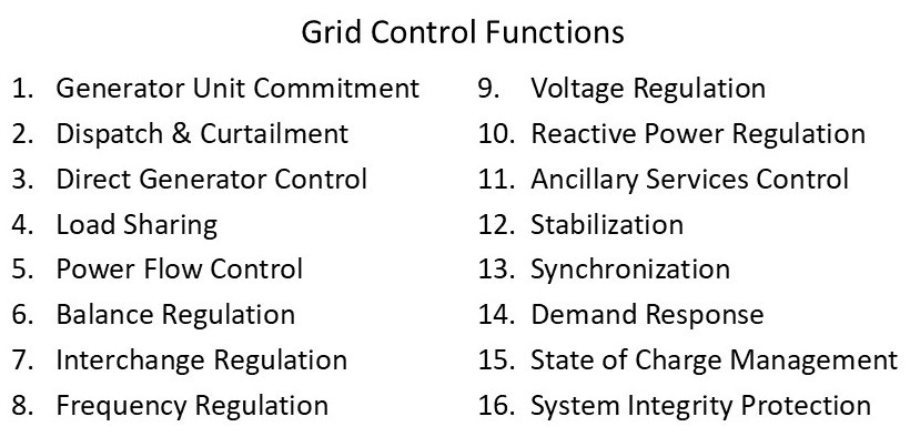
And we have not even touched upon topics like protection, black start, grid observability, power quality, ancillary services, utility communications, electricity markets, and a whole host of distribution level issues. It is no wonder that the Eastern Interconnection in the US has been described as the most complex machine ever built.