What Is Better Than Optimal?

Sometimes a little less is a lot more.

My, doesn’t the grid chattering class just love “optimal” solutions! So much so that the discussion around Distributed Energy Resources (DER) and grid transformation in the US often relies upon a magic box¹ labeled “Optimization” to make fast stochastic balancing work in Whiteboard Flatland electric grids. According to its proponents, it will coordinate tens of millions of grid-connected devices, unlock loads of latent value, and avoid the need for grid infrastructure investment. Unfortunately, in practice such optimal balancing solutions are brittle, meaning that a change in underlying conditions can make the formerly optimal solution break down, even to the point of system failure.

Not that kind of brittle. Well, ok, sorta.

First, a few maxims about optimization:

• “Optimum” does not mean ideal, it means “the best available compromise, given the constraints.”

• There are conditions under which an optimum may not exist.

• An optimum might exist (from a math standpoint), but not be feasible to implement.

• Optima can be broad and shallow, in which case being off optimum a bit makes very little difference in outcomes. Or, optima can be sharp, in which case a slight shift in operating point can make a large difference in outcomes.

• Optima may often be found right at the border between the feasible solution set and non-feasible solutions.

• A slight external condition shift can invalidate an “optimal” solution.

Consider the linear programming problem to help visualize these last two points: a slight shift in conditions can leave a formerly optimal solution outside the bounds of feasibility, as the figure below illustrates.

A slight condition change can break the system.

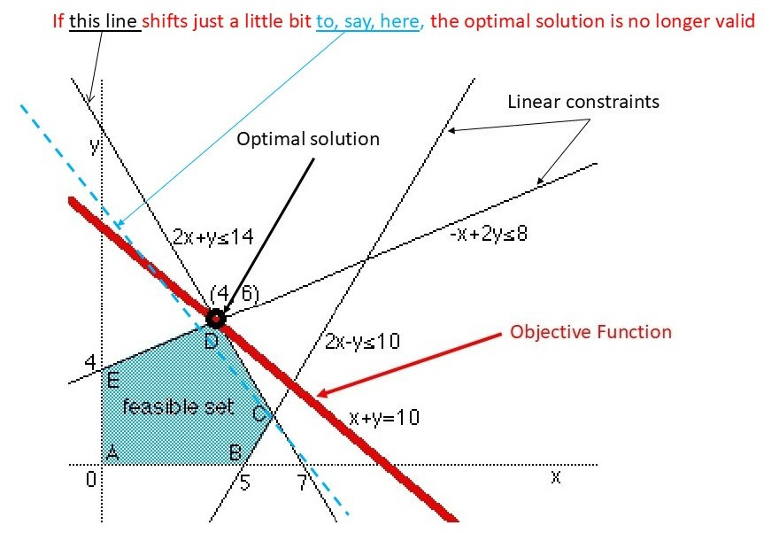
The sharper the optimum is, as compared to other solutions (an economist might say the more value it extracts), the more sensitive to condition perturbations it tends to be. So, for a sharp optimum, the chances are greater that a shift in underlying conditions (or an incorrect representation of the constraint) will cause the presumably optimal solution to fall off the optimization peak or outside the set of feasible solutions. The error can have severe consequences in an operational environment.

In other words, optima that make the biggest differences can also be the most brittle.

So then, what is better than optimal?

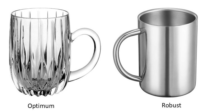
Rather than seeking the holy grail of an optimal solution, it is often better to seek a robust solution.² A robust solution is one that is relatively insensitive to variations in exogenous factors and model parameters. Such a solution will be suboptimal from the standpoint of traditional grid techno-economic objectives but will be superior to the traditional “optimal” solution under conditions of volatility, subsystem or component failure, and external system stress. In essence, we are introducing a new criterion into the problem, namely the need for the solution to be resilient.³ Once that criterion is taken into account, the new robust solution becomes stronger than the traditional techno-economic optimal solution, hence, “Better Than Optimal.”⁴

So where is this better solution to be found? Right in the neighborhood of the traditional optimal solution. Generally, optimization problems have what is known as a feasible set of solutions - ones that may satisfy the problem constraints and can be realized (implemented). Among the feasible solutions, there may be one particular solution that extremizes an objective function (setting aside the issue of local vs. global optima for the moment). Identifying the feasible solution set may in itself be difficult, and the process of locating the optimum within that set can be computationally demanding to the point of scaling unsustainably as the number of elements (such as DER devices) increases.

Rather than seeking and using the “optimal” solution, we can choose another point from the feasible solution set that is better from the standpoint of robustness. In fact, since we are choosing for robustness rather than pure extremization, there are likely many candidates to be found in the vicinity of the pure optimum - in other words, on a broader but slightly less than optimum curve, or slightly more interior to the feasible solution set than the traditional optimum. Such solutions can be easier to find than the theoretical optimum and the incremental loss of value due to being slightly off-optimal can be kept small. The idea here is to trade off the small incremental advantage of the theoretically optimal but brittle solution for the improved resilience of the less-optimal solution.

Don’t let slavish devotion to the dainty concept of optimality prevent you from using the durable solution that consistently gets the job done.

Electricity delivery is a job, not a dinner party.

Remember: robust solution > pure optimal solution. This math is on the final.

1. Magic box thinking (all too common among the grid chattering class) is related to the issue of reification.

2. In control theory there is a thing called robust control, which addresses this issue for control of physical systems. The math is formidable, but don’t worry, it won’t be on the final exam.

3. We defined resilience for the grid to have three parts. Robustness fits into the second part: ability to withstand stress without failing.

4. Yes, I know about Nassim Nicholas Taleb, but we are being practical here.